V2 Is Coming and It's Bringing Bayes with It. Our Findings on XGBoost.

When I started this project, I was operating on a personal hypothesis I'd had for a couple of years while modeling sports: since baseball has the highest variance of any major sport, introducing overly complex modeling techniques would likely lead to overfitting and, ultimately, worse performance.

I chose expected runs as the main output metric for two reasons: A) expected runs translate naturally via distributions like Poisson or negative binomial into win probabilities, making the model easier to evaluate, and B) they can also directly inform totals (over/under) predictions.

After seeing some success using tree-based models, specifically XGBoost, to predict xR-type outputs in other sports (mainly hockey), I decided to apply the same approach to baseball (my favorite sport), handpicking the features I considered most informative.

Even though I was aiming for a relatively simple approach, there were still a few key challenges to address, mainly deriving win probabilities correctly and calibration, since XGBoost is notoriously uncalibrated out of the box.

I approached the win probability problem with a negative binomial distribution rather than Poisson. Poisson assumes that variance equals mean, while real baseball scoring environments are heavily overdispersed and tend to cluster.

As for calibration, I was looking to achieve reasonable alignment between the model's confidence and actual win percentages. In other words, if the home team has a 60% win probability, then it should win roughly 60% of the time.

After a bit of research this brought me to isotonic regression, since it maps predicted probabilities to real observed frequencies and is non-parametric (we don't have to commit to a functional form).

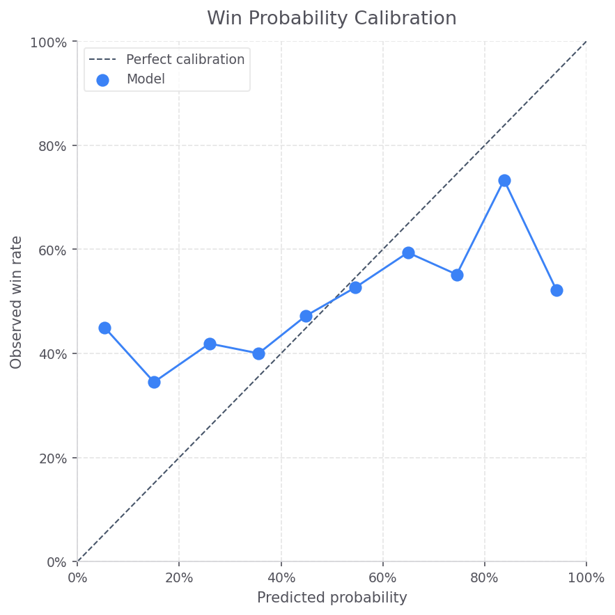
I later regretted this decision somewhat, since isotonic regression can overfit aggressively on smaller samples.

After testing on the first month of the season and evaluating against sharp betting markets, the initial betting results looked encouraging:

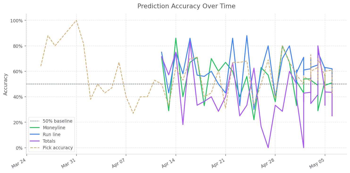
ROI was positive across several betting segments, particularly underdogs and run lines:

Category	ROI	Record
Favorites	+4.2%	29-23
Underdogs	+22.0%	63-59
Run Line	+10.0%	110-67
Overs	-1.6%	43-47
Unders	-23.2%	28-41

Average line on underdog bets: +111

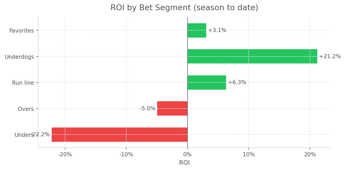
However, betting performance over a one-month sample is extremely noisy and easy to misinterpret. Positive ROI alone does not necessarily imply that the underlying probability estimates are strong.

The more important story appeared in the probability performance metrics themselves.

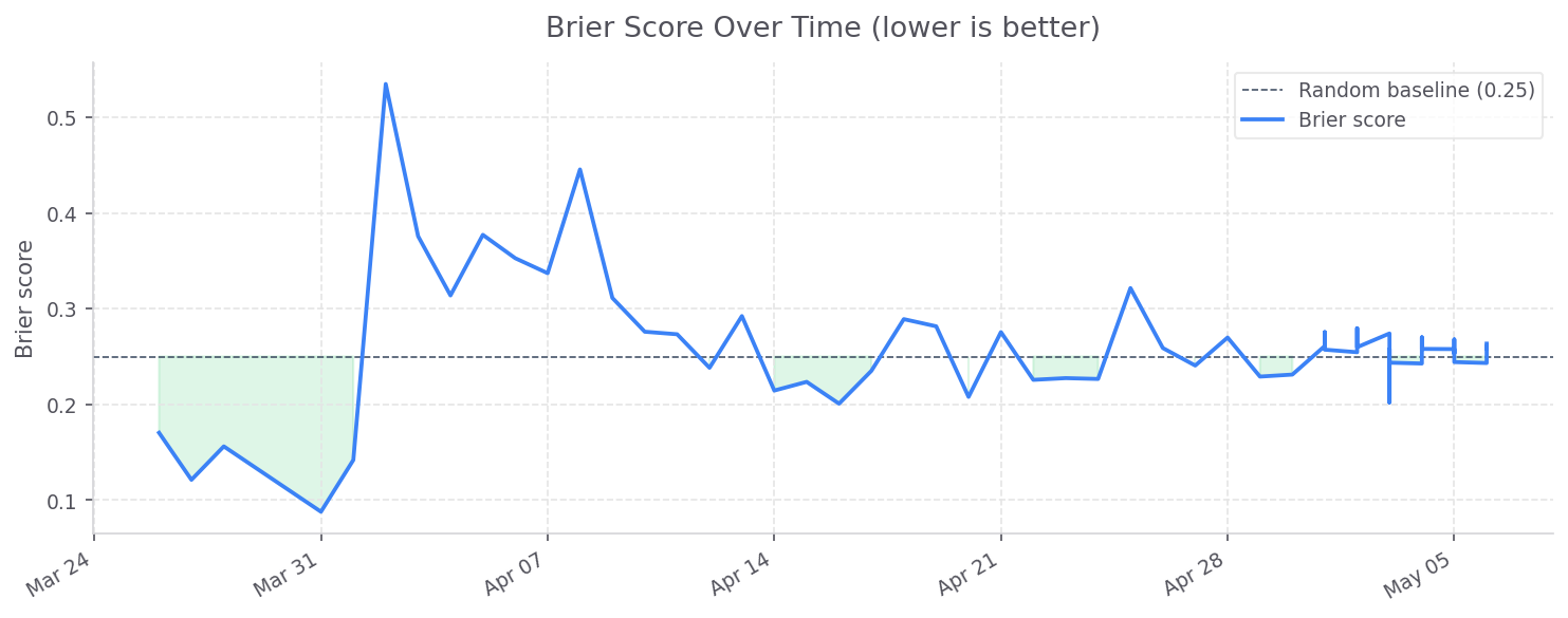
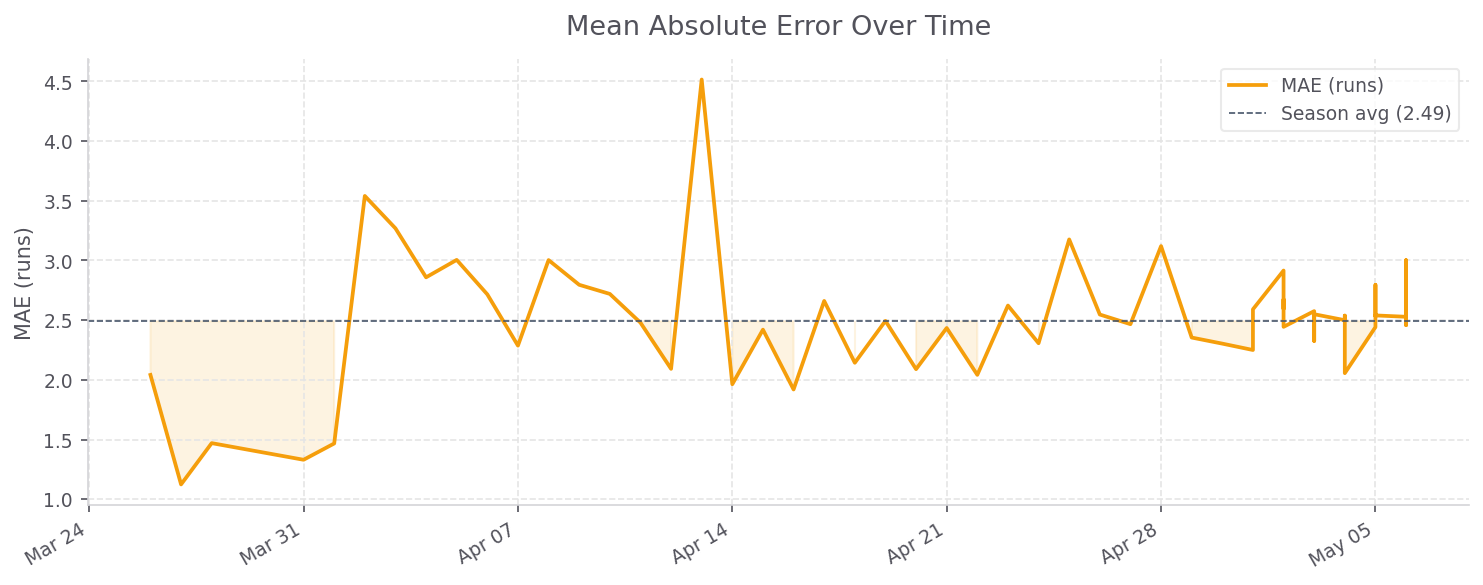
Despite some positive betting outcomes, the model's probability predictions were only marginally better than random.

Brier score, which measures calibration quality, suggested that the model outputs were only negligibly better than coin-flip probabilities. Meanwhile, MAE settled around 2.4 runs of average error, which is a respectable baseline for baseball scoring prediction.

The real issue wasn't the 2.4 runs of MAE on its own. It was that the whole setup is locked to a point estimate, so even when the model picks the right side of a bet, it has nothing to say about how the run distribution is actually shaped. That matters most on totals, where the line is asking a distributional question and a single number can't answer it.

That realization pushed me toward a simulation-based Bayesian framework for v2.

The Beauty of Bayes

Back when I was an undergrad with a growing interest in probability and statistics, looking for alternatives to the limitations of frequentist modeling, I was drawn to the beauty of the way Bayesian methods formalize how rational minds should update beliefs, effectively describing how learning works by adjusting through new data. I particularly liked the self-correcting nature of Bayes' theorem and the graceful handling of initially limited data. Hence, hierarchical bayesian.

Bayesian modeling in one paragraph:

Instead of finding a single best parameter value, we treat parameters as random variables and estimate their posterior distribution given the observed data. We start with a prior (what we believe before seeing data), combine it with the likelihood (how well different parameter values explain the observed outcomes), and arrive at a posterior (what we believe after observing the data). The posterior gives us not just a point estimate, but an explicit measure of uncertainty.

"Hierarchical" means parameters are nested. Each individual batter has their own skill profile, but those skills are drawn from a shared population distribution. This gives us partial pooling: a rookie with 50 plate appearances gets shrunk heavily toward the league average because we do not yet trust the sample, while a veteran with 5,000 plate appearances barely shrinks at all because the observed data dominates the prior. XGBoost has no equivalent mechanism; it treats every observation independently.

Concretely, v2 models each plate appearance as a probabilistic interaction between batter skill, pitcher skill, platoon effects, and park context.

The model itself is a hierarchical multinomial-logit over eight outcome cells per plate appearance: strikeout, walk, hit-by-pitch, single, double, triple, home run, and out-in-play. (An earlier version of this post called it a Dirichlet-Multinomial. It is not: the actor effects are Normal on the logit scale, which makes the outcome probabilities logistic-normal, and no Dirichlet prior is involved.)

For each batter, we estimate a seven-dimensional vector of additive logit offsets (with "out" as the reference category). Pitchers receive the same treatment, with separate variance structures for starters and relievers. The model also includes platoon split adjustments and park-level residual effects on wOBA.

When a specific batter faces a specific pitcher, the outcome probabilities are generated by softmaxing the sum of:

• League-average logits (the intercept)
• Batter logit offsets for the relevant platoon split
• Pitcher logit offsets
• Park effects

The Simulator: Per-Plate-Appearance Monte Carlo

Once we have posterior estimates for batter skill, pitcher skill, and park effects, the simulator plays out each game one plate appearance at a time, running 10,000+ simulations per matchup.

The output is not a single projected score, but a full joint distribution over (home_runs, away_runs), from which moneyline, run line, and totals probabilities can be derived directly.

This removes the need for a manually imposed negative binomial assumption and avoids unrealistic independence assumptions between teams. Instead, the simulator allows scoring correlation structures to emerge naturally from the interaction between lineups, pitchers, bullpen usage, and game context.

Why This Is Better Than V1

A few concrete things v2 can do that v1 could not:

• Lineup-aware predictions. v1 relied on team-level batting splits, meaning a team with its full starting lineup received nearly the same prediction as a banged up or resting lineup. v2 incorporates the actual posted lineup directly into the simulation.

• Distribution-aware outputs. v1 focused primarily on point estimates and assumed run distributions afterward. v2 generates the scoring distribution itself through simulation.

• Calibrated uncertainty. The posterior distributions naturally provide credible intervals and uncertainty estimates for every modeled quantity.

• Extensibility. Adding weather effects, umpire tendencies, or batter-pitcher interaction terms simply means extending the generative model itself rather than rebuilding an entirely new feature-engineered pipeline.

• Better structural realism. Baseball games are sequential, interaction-heavy processes. Modeling them at the plate-appearance level is simply a more faithful representation of how run environments actually emerge.